Rotterdam Breast Cancer: From Confounding to Overlap Weighting

日本語 · 中文 · English

GitHub · Code / コード / 代码

Author: Ziyin Wu (WU ZIYIN). Based on the final presentation of August 18, 2026 and its accompanying R code. This is a personal educational solution, not an official answer, a peer-reviewed study, or medical advice. The public documentation was organized and translated with AI assistance; the presentation code is preserved separately.

Open the trilingual HTML slides — a reconstructed public teaching edition, with institutional, examination and personal details removed from the cover; not a page-for-page copy of the original PDF.

Reproduction and publication record · Validate with python3 analysis/verify.py.

1. Question and scope

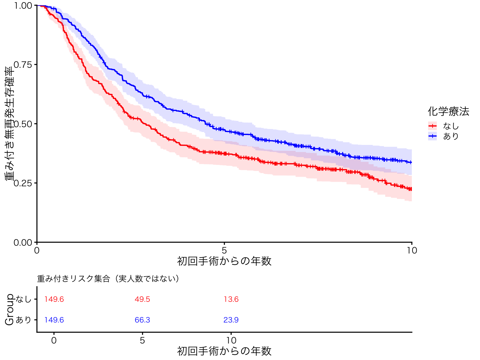
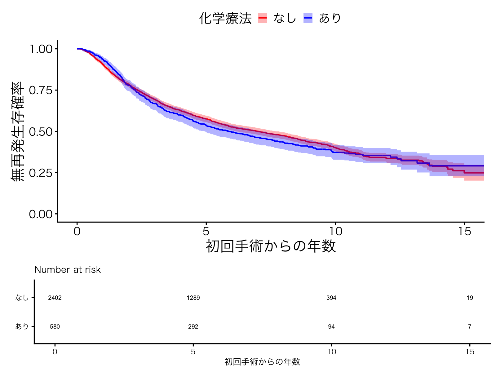
Using survival::rotterdam, compare recurrence-free survival (RFS) between patients recorded as receiving versus not receiving chemotherapy, and explain why an observational comparison is not automatically a treatment effect. The registry contains 2,982 primary breast cancer patients. Time zero is initial surgery; RFS ends at the first observed recurrence or death. The final presentation reports an unadjusted whole-cohort comparison, followed by an additional adjusted analysis with a different target population.

2. Reproduce

From the repository root, in R install the required packages if needed:

install.packages(c("survival", "ggplot2", "survminer", "WeightIt",
                  "cobalt", "adjustedCurves", "pammtools"))

Rscript analysis/run.R > results/run.log 2>&1

analysis/survival.R is the original final-presentation script, not the earlier exploratory audit. analysis/run.R adds a graphics device and CSV/session-information exports without changing statistical formulas. It writes only under results/ when run as above. The bootstrap uses seed 20260717, 500 patient-level resamples, and one core. Software versions are in sessionInfo; installed package versions can change numerical results. The original plotting code specifies Hiragino Sans, available on macOS. Other platforms may need a Japanese font substitution for figures; this does not change the statistical models.

Data are loaded from the R package, not copied from a different Rotterdam/Stata dataset. Patient-level CSVs produced at runtime are excluded from publication. No admission documents, third-party paper PDFs, lecture slides, or backup files are included.

3. Analysis workflow

1. Define RFS correctly. Set recurrence time to infinity when no recurrence was observed, and death time to infinity when no death was observed. Their minimum defines an event when finite. If neither occurred, use the maximum of the two recorded follow-up times, following the assignment’s supplied definition. Convert days to years using 365.25. Do not take an unqualified minimum of two follow-up columns.
2. Audit the data. Check 2,982 unique patients, no missing values, 580 chemotherapy recipients and 2,402 nonrecipients, 1,713 composite events and 1,269 censored observations.
3. Unadjusted comparison. Estimate Kaplan–Meier curves with log–log confidence intervals; use the log-rank test over the full follow-up. Report the five-year survival difference with a normal approximation using independent-group Greenwood standard errors. A nonsignificant test is not evidence of equivalence.
4. Explain confounding and overlap. Treatment was not randomized. Patient background is associated with both treatment selection and prognosis. All 580 treated patients are node-positive; the 1,436 node-negative patients include no treated comparator. Thus, an empirical positivity problem prevents a supported treated-versus-untreated comparison in that stratum.
5. Change the target explicitly. Restrict the additional analysis to 1,546 node-positive patients (966 untreated, 580 treated), then target their overlap population, not the original whole cohort.
6. Fit a propensity score. Logistic regression uses natural splines for age (4 df), log(1 + nodes), log(1 + ER), and log(1 + PgR) (3 df each), plus menopausal status, tumor size, and grade. Surgery year and hormone treatment are not included in this final model. Their omission is not proof that they could not confound the association.
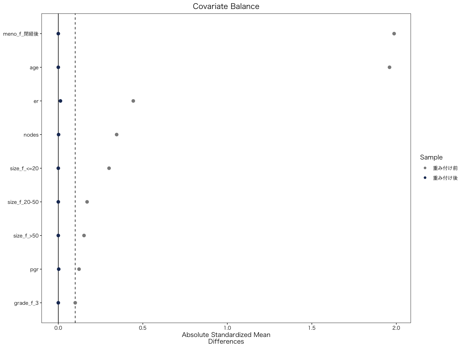
7. Overlap weighting. With propensity score e(L), treated patients receive weight 1 − e(L), untreated patients e(L). WeightIt::weightit(method="glm", estimand="ATO") targets a population whose covariate density is proportional to e(L)[1 − e(L)]f(L).
8. Diagnostics. Check standardized mean differences before/after weighting and effective sample sizes (ESS). The reproduced ESS is 277.81 untreated and 328.31 treated; maximum absolute reported post-weighting SMD is about 0.0126. Good measured balance does not establish absence of unmeasured confounding.
9. Adjusted survival and RMST. Use adjustedCurves::adjustedsurv(method="iptw_km", estimand="ATO"). Despite the method name, these are overlap weights, not ATE inverse-probability weights. Re-estimate the propensity score and weights within every bootstrap sample. Integrate survival up to five years for restricted mean survival time (RMST); the code also exports ten-year summaries.

4. Final five-year results

All contrasts below are chemotherapy minus no chemotherapy. RFS differences use percentage points, not relative percentages. Brackets are 95% confidence intervals.

Analysis / measure	No chemotherapy	Chemotherapy	Difference
Whole-cohort unadjusted RFS	57.5% [55.5, 59.5]	53.7% [49.5, 57.7]	−3.8 pp [−8.4, +0.7]
Node-positive overlap-population RFS	37.4% [32.4, 42.8]	47.4% [42.4, 52.7]	+10.0 pp [+2.4, +17.7]
Node-positive overlap-population RMST	3.00 years [2.80, 3.20]	3.53 years [3.36, 3.70]	+194 days [+98, +289]

The unadjusted full-follow-up log-rank p-value is 0.4078 (0.408 in the slides). Exact exported values and the execution log are in results. The original slides round the RMST difference to whole days.

5. How to interpret the apparent reversal

The crude result does not show that chemotherapy harms patients, and the adjusted result does not prove that chemotherapy causes benefit. Treatment groups differed substantially at baseline. Furthermore, both adjustment and the target population change between the two analyses; the sign change cannot be attributed solely to removal of confounding.

A plain-language analogy: ice-cream purchases and heatstroke may rise together because hot weather increases both. Similarly, patient characteristics can influence both treatment choice and recurrence/death risk. Weighting makes the measured backgrounds more comparable, but cannot recover unmeasured variables or create evidence for a treatment group absent from a stratum.

The +194-day RMST contrast means a difference in average recurrence-free time accumulated within the first five years, in the node-positive overlap population. It is not a gain in total life expectancy and does not predict an individual patient’s benefit.

6. Limitations and methodological history

• This is historical observational data. Unmeasured confounding, treatment timing, treatment heterogeneity, and censoring assumptions limit interpretation. Surgery is time zero while chemotherapy is represented by a recorded indicator; the analysis does not establish time-aligned treatment assignment or rule out immortal-time bias.
• A causal interpretation would require defensible consistency, exchangeability/no unmeasured confounding, positivity for the target population, and appropriate censoring assumptions. Consistency is an assumption, not something that always holds automatically.
• The supplied RFS censoring convention is reproduced faithfully; its suitability depends on the underlying follow-up process.
• Bootstrap execution emitted 23 propensity-score separation warnings in the verified environment. They were recorded, not silently discarded. The exported 5/10-year group summaries contain 500 bootstrap contributions, but that does not remove potential inference instability.
• The presentation appendix discusses exploratory Cox proportional-hazards diagnostics and extreme ATE-IPTW weights. Those analyses are not implemented by the final survival.R and are not claimed as reproduced results here. They explain the methodological exploration, not a second final model.
• Public explanatory text clarifies percentage points and causal assumptions; it is not a verbatim republication of every slide. Original slides are not redistributed because they also contain institutional presentation material and lecture-derived content.

References

• R survival package, Rotterdam dataset documentation.
• Royston P, Altman DG. External validation of a Cox prognostic model: principles and methods. BMC Med Res Methodol. 2013;13:33. https://doi.org/10.1186/1471-2288-13-33
• Elkin EB et al. Adjuvant chemotherapy and survival in older women with hormone receptor-negative breast cancer. J Clin Oncol. 2006;24:2757–2764. https://doi.org/10.1200/JCO.2005.03.6053
• Du XL et al. Effectiveness of adjuvant chemotherapy for node-positive operable breast cancer in older women. J Gerontol A. 2005;60:1137–1144. https://doi.org/10.1093/gerona/60.9.1137
• Li F, Morgan KL, Zaslavsky AM. Balancing covariates via propensity score weighting. JASA. 2018;113:390–400. https://doi.org/10.1080/01621459.2016.1260466
• Li F, Thomas LE, Li F. Addressing extreme propensity scores via the overlap weights. Am J Epidemiol. 2019;188:250–257. https://doi.org/10.1093/aje/kwy201
• Denz R, Klaaßen-Mielke R, Timmesfeld N. A comparison of different methods to adjust survival curves for confounders. Stat Med. 2023;42:1461–1479. https://doi.org/10.1002/sim.9681
• Royston P, Parmar MKB. Restricted mean survival time: an alternative to the hazard ratio. BMC Med Res Methodol. 2013;13:152. https://doi.org/10.1186/1471-2288-13-152
• Hernán MA, Robins JM. Causal Inference: What If.

For educational reference and critical examination, not for copying into an examination submission. Code and documentation retain their authors’ rights; no blanket license is granted over third-party datasets or references.